Showing posts with label Programming. Show all posts

Thursday, 24 January 2013

Direct3DX9NotFoundException Creating a Direct3D Device With SlimDX


Yet another note for future reference. If you are using SlimDX, and you get the exception:


SlimDX.Direct3D9.Direct3DX9NotFoundException was unhandled
Message=Direct3DX 9 was not found. Please install the latest
DirectX end-user redistributable package from Microsoft.
Source=SlimDX
StackTrace:
at SlimDX.Direct3D9.Direct3D..ctor()
InnerException: System.Runtime.InteropServices.SEHException
Message=External component has thrown an exception.
Source=SlimDX
ErrorCode=-2147467259
StackTrace:
at D3DXCheckVersion(UInt32 , UInt32 )
at SlimDX.Direct3D9.Direct3D..ctor()
InnerException:


when trying to create a SlimDX.Direct3D9.Direct3D object, most likely you will be able to solve this by placing D3DX9_43.dll into your output folder. Please note that the proper solution would be to install the full DirectX 9 runtime into your system, but it may be too much for some quick testing.


A similar error may occur when using SharpDX, but in SharpDX's case, the error message will be much more helpful and actually tell you what is missing.

Tuesday, 15 January 2013

The command "sn -Ra ... :VCEnd" exited with code 1

For today, a quick note for future reference. If you have a C++/CLI project and you are getting the error


MSB3073: The command "sn -Ra "YourProject.dll" "YourKey.snk"
:VCEnd" exited with code 1. C:\Program Files (x86)\MSBuild\Microsoft.Cpp\v4.0\Microsoft.CppCommon.targets


Then try adding the following two lines to your AssemblyInfo.cpp


[assembly:AssemblyKeyFileAttribute("application_key.snk")];
[assembly:AssemblyDelaySignAttribute(true)];


and check if it solves the issue. Hope this can be useful for others facing this same situation I encountered some days earlier.

Thursday, 5 April 2012

Quadratic Programming in C#


I have manually translated and adapted the QuadProg solver for quadratic programming problems made by Berwin A. Turlach. His code was originally published under the GNU Library License, which has now been superseded by the GNU Lesser License. This adapted version honors the original work and is thus distributed under the same license.


Introduction


Despite the name, the terms linear or quadratic programming have little resemblance to the set of activities most people now know as programming. Those terms usually usually refers to a specific set of function optimization methods, i.e. methods which can be used to determine the maximum or minimum points of special kinds of functions under a given number of solution constraints. For example, suppose we would like to determine the minimum value of the function:


f(x, y) = 2x + y + 4


Under the constraints that x and y must be non-negative (i.e. either positive or zero). This may seem fairly simple and trivial, but remember that practical linear programming problems may have hundreds or even thousands of variables and possibly million constraints.


When the problem to be solved involves a quadratic function instead of a linear function, but still presents linear constraints, this problem can be cast as a quadratic programming problem. Quadratic functions are polynomial functions in each each term may have at most a total degree of 2. For example, consider the function


f(x, y, z) = 2x² + 5xy + y² - z² + x – 5.


Now let's check the sum of the degrees for each variable on the polynomial terms. We start by writing the missing terms of the polynomial


f(x, y, z) = 2 x2y0z0 + 5 x1y1z0 + 2 x0y2z0 - x0y0z2 + x1y0z0 - 5 x0y0z0


and then proceed to check the sum of the degrees at each term. In the first term, 2+0+0 = 2. For the second, 1+1+0 = 2, and so on. Those functions have a nice property that they can be expressed in a matrix form


f(x) = 1/2 xT Q x + cTx.


Here, x and c are vectors. The matrix Q is a symmetric matrix specifying how the variables combine in the quadratic terms of the function. If this matrix is positive definite, then the function is convex, and the optimization has a single, unique optimum (we say it has a global optimum). The coefficients c specify the linear terms of our function.


Source code


The available source code is based on a translation of the Fortran code written by Berwin A. Turlach. However, some modifications have been made. Fortran uses column-major ordering for matrices, meaning that matrices are stored in memory in sequential order of column elements. Almost all other languages use row-major ordering, including C, C++, Java and C#. In order to improve data locality, I have modified the code to use the transpose of the original matrices D and A. I have also modified the QP formulation adopted in the Goldfarb and Idnani paper to reflect the form presented in the introduction.


This code is part of the Accord.NET Framework. However, the version available in this blog post will most likely not be the most recently, updated, fixed and enhanced version of the code. For the latest version, be sure to download the latest version of the framework on the project site or through a NuGet package.


Using the code


The first step in solving a quadratic programming problem is, well, specifying the problem. To specify a quadratic programming problem, one would need two components: a matrix D describing the relationship between the quadratic terms, and a vector d describing the linear terms. Perhaps this would work better with an example.


Suppose we are trying to solve a minimization problem. Given a function, the goal in such problems is to find the correct set of function arguments which would result in the minimum possible value for the function. An example of a quadratic minimization problem is given below:


min f(x, y) = 2x² - xy + 4y² - 5x – 6y


subject to the constraints:


x - y = 5


x = 10


wolfram
(generated with Wolfram Alpha)


However, note that this problem involves a set of constraints. The required solution for this minimization problem is required to lie in the interval specified by the constraints. More specifically, any x and y pair candidate for being a minimal of the function must respect the relations x - y = 5 and x >= 10. Thus, instead of lying in the unconstrained minimum of the function surface shown above, the solution lies slightly off the center of the surface. This is an obvious easy problem to solve manually, but it will fit for this demonstration.


wolfram2


As it can be seen (and also live demonstrated by asking Wolfram Alpha) the solution lies on the point (10,5), and the constrained minimum of the function is given by 170. So, now that we know what a quadratic programming problem looks like, how can we actually solve it?


Specifying the objective function


The first step in solving a quadratic programming problem is to specify the objective function. Using this code, there are three ways to specify it. Each of them has their own advantages and disadvantages.


1. Manually specifying the QP matrix.


This is the most common approach for numerical software, and probably the most cumbersome for the user. The problem matrix has to be specified manually. This matrix is sometimes denoted Q, D or H as it actually denotes the Hessian matrix for the problem.


The matrix Q is used to describe the quadratic terms of our problem. It is a n x n matrix, in which n corresponds to the number of variables in our problem, covering all possible combinations of variables. Recall our example given on the start of this section. We have 2 variables, x and y. Thus, our matrix Q is 2 x 2. The possible combinations for x and y are expressed in the table below.


x

y

x

x*x

x*y

y

y*x

y*y


To form our matrix Q, we can take all coefficients associated with each pair mentioned on the table above. The diagonal elements should also be multiplied by two (this is actually because the matrix is the Hessian matrix of the problem: it is the matrix of all second-order derivatives for the function. Since we have only at most quadratic terms, the elementary power rule of derivation “drops” the ² from the x² and y² terms – I think a mathematician would hit me with a stick for explaining it like this, but it serves well for a quick, non-technical explanation).


Remember our quadratic terms were 2x²  - 1xy + 4y². Writing the terms on their proper position and differentiating, we have:


As it can be seen, the matrix is also symmetric (and often, but not always, positive definite). The next step, more trivial, is to write a vector d containing the linear terms. The linear terms are –5x –6y, and thus our vector d can be given by:


Therefore our C# code can be created like this:


    double[,] Q =
{
{ +4, -1 },
{ -1, +8 },
};

double[] d =
{
-5,
-6
};


2. Using lambda expressions


This approach is a bit more intuitive and less error prone. However, it involves lambdas functions and some people find it hard to follow them. Another disadvantage is that we will lose the edit & continue debugging ability of visual studio. The advantage is that the compiler may catch some obvious syntax errors automatically.


    double x = 0, y = 0;

QuadraticObjectiveFunction f = // 2x² - xy + 4y² - 5x - 6y
new QuadraticObjectiveFunction(() => 2*(x*x) - (x*y) + 4*(y*y) - 5*x - 6*y);


Note that the x and y variables could have been initialized to any value. They are only used as symbols, and not used in any computations.


3. Using text strings


This approach is more intuitive but a bit more error prone. The function can be specified using strings, as in a standard mathematical formula. However, since all we have are strings, there is no way to enforce static, compile time checking.


    QuadraticObjectiveFunction f = 
new QuadraticObjectiveFunction("2x² - xy + 4y² - 5x - 6y");


Couldn’t be easier.


Specifying the constraints


The next step in specifying a quadratic programming problem is to specify the constraints. The constraints can be specified in almost the same way as the objective function.


1. Manually specifying the constraints matrix


The first option is to manually specify the constraints matrix A and vector b. The constraint matrix expresses the way the variables should be combined when compared to corresponding value on vector b. It is possible to specify either equality constraints or inequality constraints. The formulation used in this code is slightly different from the one used in Turlach’s original implementation. The constraints are supposed to be in the form:


A1 x = b1


A2 x = b2


This means that each line of matrix A expresses a possible combination of variables x which should be compared to the corresponding line of b. An integer variable m can be specified to denote how many of the first rows of matrix A should be treated as equalities rather than inequalities. Recall that in our example the constraints are given by 1x -1y = 5 and 1x = 10. Lets write this down in a tabular form:


#

x

y

?

b

q1

1

-1

=

5

q2

1

0

=

10


Thus our matrix A and vector b can be specified as:


And not forgetting that m = 1, because the first constraint is actually an equality.


2. Using classes and objects


A more natural way to specify constraints is using the classes and objects of the Accord.NET Framework. The LinearConstraint class allows one to specify a single constraint using an object-oriented approach. It doesn’t have the most intuitive usage on earth, but has much more expressiveness. It can also be read aloud, it that adds anything! :-)


    List<LinearConstraint> list = new List<LinearConstraint>();

list.Add(new LinearConstraint(numberOfVariables: 1)
{
VariablesAtIndices = new[] { 0 }, // index 0 (x)
ShouldBe = ConstraintType.GreaterThanOrEqualTo,
Value = 10
});

list.Add(new LinearConstraint(numberOfVariables: 2)
{
VariablesAtIndices = new int[] { 0, 1 }, // index 0 (x) and index 1 (y)
CombinedAs = new double[] { 1, -1 }, // when combined as 1x -1y
ShouldBe = ConstraintType.EqualTo,
Value = 5
});


The specification is centered around the notion that variables are numbered and have an associated index. For example, x is the zero-th variable of the problem. Thus x has an index of 0 and y has an index of 1. So for example, reading aloud the last constraint, it is possible to express how the variables at indices 0 and 1, when combined as 1x and –1y, should be equal to value 5.


2. Using lambda expressions


A more intuitive way to express constraints is again using lambda expressions. And again the problems are the same: some people find it hard to follow and we lose edit & continue.


    var constraints = new List<LinearConstraint>();
constraints.Add(new LinearConstraint(f, () => x - y == 5));
constraints.Add(new LinearConstraint(f, () => x >= 10));


3. Using text strings


Same as above, but with strings.


    var constraints = new List<LinearConstraint>();
constraints.Add(new LinearConstraint(f, "x - y = 5"));
constraints.Add(new LinearConstraint(f, "x >= 10"));


Finally, creating and solving the problem


Once we have specified what do we want, we can now ask the code for a solution. In case we have opted for manually specifying the matrix A, vector b and integer m, we can use:


    // Create the optimization problem
var solver = new GoldfarbIdnaniQuadraticSolver(numberOfVariables:2, A, b, m);


In case we have opted for creating a list of constraints instead, we can use:


    // Create our optimization problem
var solver = new GoldfarbIdnaniQuadraticSolver(numberOfVariables: 2, constraints: list);


After the solver object has been created, we can call Minimize() to solve the problem. In case we have opted for manually specifying Q and d, we can use:


    // Attempt to solve the problem
double minimumValue = solver.Minimize(Q, d);


And in case we have opted for creating a QuadraticObjectiveFunction object, we can use:


    // Attempt to solve the problem
double minimumValue = target.Minimize(f);


In either case, the solution will be available in the Solution property of the solver object, and will be given by:


    double value = solver.Value;    // f(x,y) = 170
double x = solver.Solution[0]; // x = 10
double y = solver.Solution[1]; // y = 5


Sample application


The Accord.NET Framework now includes a sample application demonstrating the use of the Goldfarb-Idnani Quadratic Programming Solver. It can be downloaded at the Accord.NET Framework site, and also comes together with recent versions of the framework (> 2.6).


Solver


Solver sample application included in the Accord.NET Framework.


Remarks


Because the code has been translated by hand (in contrast of using automatic translators such as f2c) there could be potential bugs in the code. I have tested the code behavior against R’s quadprog package and still didn’t find errors. But this does not mean the code is bug-free. As always, as is the case of everything else in this blog, this code is published in good faith, but I can not guarantee the correctness of everything. Please read the disclaimer for more information.


References


Wednesday, 4 January 2012

Decision Trees in C#

Decision trees are simple predictive models which map input attributes to a target value using simple conditional rules. Trees are commonly used in problems whose solutions must be readily understandable or explainable by humans, such as in computer-aided diagnostics and credit analysis.

treeIntroduction

Decision Trees give a direct and intuitive way for obtaining the classification of a new instance from a set of simple rules. Because of this characteristic, decision trees find wide use in situations in which the interpretation of the obtained results and of the reasoning process is crucial, such as in computer-aided diagnostics (CAD) and in financial credit analysis. Consumer credit analysis is an interesting example because, in many countries, one can not simply reject credit without giving a justification, justification of which is trivial to extract from a decision tree.

The tree on the right has been generated using the Context Free software based on the grammar shared by davdrn.

Learning decision trees

Decision trees can be simply drawn by hand based on any prior knowledge the author may have. However, their real power becomes apparent when trees are learned automatically, through some learning algorithm.

The most notable and classics examples to decision tree learning are the algorithms ID3 (Quinlan, 1986) and the C4.5 (Quinlan, 1993). Both are examples of greedy algorithms, performing local optimum decisions in the hope of producing a most general tree. Such algorithms are based on the principle of the Occam's razor, favoring simpler or smaller trees in the hope that such smaller trees could retain more generalization power. This preference is formalized through the specification of an hypothesis ordering criteria such as the information gain. The information gain measures the, as the name implies, gain of information in using each of the attributes as a next factor to consider during decision. The information gain can be defined as:

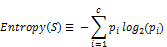
image003

image004

However, the information gain has a bias towards attributes with a high number of possible values (Mitchell, 1997). A way to overcome this bias is to select new selection attributes based on alternative criteria, such as the gain ratio (Quinlan, 1986), defined as:

image005

image006

In the GainRatio, the SplitInformation term attenuates the importance given to attributes with many, uniformly distributed, possible values.

Iterative Dichotomizer 3 (ID3)

The algorithm presented below is a slightly different version of the original ID3 algorithm as presented by Quinlan. The modifications are to support multiple output labels. In each recursion of the algorithm, the attribute which bests classifiers the set of instances (or examples, or input-output pairs, or data) is selected according to some selection criteria, such as the InfoGain or the GainRatio.

  • ID3(instances, target_attribute, attributes)
    • Create a new root node to the tree.
    • If all instances have the target_attribute belonging to the same class c,
      • Return the tree with single root node with label c.
    • If attributes is empty, then
      • Return the tree with single root node with the most common label of the target_attribute in instances.
    • Else
      • A ← the attribute in attributes which best classifies instances
      • root decision attribute ← A
      • Foreach possible value vi of A,
        • Add a new ramification below root, corresponding to the test A = vi
        • Let instancesvi be the subset of instances with the value vi for A
        • If instancesvi is empty then
          • Below this ramification, add a new leaf node with the most common value of target_attribute in instances.
        • Else below this ramification, add the subtree given by the recursion:
                  ID3(instancesvi, target_attribute, attributes – { A })
    • End
  • Return root

Difficulties and disadvantages of decision tree learning

Despite relying on the Occam’s Razor to guide the learning, neither ID3 or C4.5 algorithms are not guaranteed to produce the smaller or more general tree possible. This happens because their learning is based solely on heuristics and not in truly optimality criteria. The following example, from (Esmeir & Markovitch, 2007) illustrates the learning of the concept xor (exclusive or) by the ID3 algorithm. In this example, A3 and A4 are irrelevant attributes, having absolutely no influence on the target answer. However, yet being irrelevant, ID3 will select one of them to belong to the tree. In fact, ID3 will select the irrelevant attribute A4 to be the root of the learned tree.


A1 A2 A3 A4 label
1 0 0 1 +
0 1 0 0 +
0 0 0 0 -
1 1 0 0 -
0 1 1 1 +
0 0 1 1 -
1 0 1 1 +


image


One complication of decision tree learning is that the problem to find the smaller consistent tree (in the sense of classifying correctly all training samples) is known to be NP-complete (Hyafil & Rivest, 1976). Moreover, the separating decision surface generated by such trees are always formed by parallel cuts alongside the attribute space axis, which could be a severely suboptimal solution (Bishop, 2007, p. 666). The example given by Bishop illustrates well this problem: for example, to separate classes whose optimum decision margin are on 45 degrees from one of the axis, it will be needed a high number of parallel cuts in comparison with a single cut on the diagonal such as could be given by any linear decision machine. Another disadvantage of traditional decision tree learning algorithms is that most methods require only a constant learning time, and, as such, do not allow for trading extra training time for a better solutions. The work of (Esmeir & Markovitch, 2007) is dedicated to overcome such problem.

The following picture shows an example on how learning by decision trees is limited to cuts parallel to the axis, as described by Bishop. The Ying-Yang classification problem is a classical example of a non-linearly separable decision problem. Decision trees, albeit not being linear classifiers, have difficulty classifying this set with simple thresholds.

data-closerdecision-closertree

Top-Left: Ying-Yang non-linear classification problem. Top-Right: Decision surface extracted by a decision tree. Bottom: Decision threshold rules extracted from the tree.

However, despite all of those shortcomings, decision trees plays major roles as base of many successful algorithms. One interesting application and of notorious success is given in the field of object detection in images. The first real-time face detecting algorithm (Viola & Jones, 2001) is based on a degenerated decision tree (also known as a cascade). The body recognition and segmentation algorithm used by the Xbox 360 gaming platform used to process depth images generated by its companion sensor Kinect is equally based on the use of decision trees (Shotton, et al., 2011). As well is the case of the FAST algorithm for interest point detection in images (Rosten & Drummond, 2006).

I should also make the note that both the Viola-Jones and the FAST algorithms are available in the Accord.NET Framework for immediate use (the Viola-Jones (HaarObjectDetector) has also been recently updated to support multiple threads, so feel free to take a look and experiment with it!).

In sum, its possible to say that great part of the applicability of decision trees came from the simple fact that they are extremely fast to evaluate. One of the reasons for this feature is being easily translated to sets of conditional instructions in a conventional computer program. The decision trees now available in the Accord.NET Framework make full use of this fact and enables the user to actually compile the decision trees to native code on-the-fly, augmenting even more its performance during classification.

Source code

The code presented in this section is actually part of the Accord.NET Framework. The Accord.NET Framework is a framework extension to the already very popular AForge.NET Framework, adding and providing new algorithms and techniques for machine learning, computer vision and even more.

The Accord.MachineLearning.DecisionTree namespace is comprised of the following classes:

  • DecisionTree, the main class representing a decision tree, with methods such as Compute to compute the tree classification given an input vector;
  • DecisionNode, the node class for the decision tree, which may or may not have children nodes contained under a collection of children represented by a DecisionBranchNodeCollection;
  • DecisionVariable, a class to specify the nature of each variable processable by the tree, such as if the variable is continuous, discrete, which are their expected or valid ranges;
  • DecisionBranchNodeCollection, a class to contain children nodes together with information about which attribute of the data should be compared with the child nodes during reasoning.


Whose relationships can be seen in the following class diagram:

class diagram

The learning algorithms available are either the ID3 algorithm discussed above, or its improved version C4.5 (which can handle continuous variables, but at this time does not yet support pruning), both proposed and published by Ross Quinlan.

learning

Despite the bit complicated look, usage is rather simple as it will be shown in the next section.

Using the code

Consider, for example, the famous Play Tennis example by Tom Mitchell (1998):


  DataTable data = new DataTable("Mitchell's Tennis Example");
 
  data.Columns.Add("Day", "Outlook", "Temperature", "Humidity", "Wind", "PlayTennis");
 
  data.Rows.Add(   "D1",   "Sunny",      "Hot",       "High",   "Weak",    "No" );
  data.Rows.Add(   "D2",   "Sunny",      "Hot",       "High""Strong",   "No" );
  data.Rows.Add(   "D3""Overcast",    "Hot",       "High",   "Weak",    "Yes" );
  data.Rows.Add(   "D4",   "Rain",       "Mild",      "High",   "Weak",    "Yes" );
  data.Rows.Add(   "D5",   "Rain",       "Cool",     "Normal""Weak",    "Yes" );
  data.Rows.Add(   "D6",   "Rain",       "Cool",     "Normal", "Strong",   "No" );
  data.Rows.Add(   "D7""Overcast",    "Cool",     "Normal", "Strong",   "Yes" );
  data.Rows.Add(   "D8",   "Sunny",      "Mild",      "High",   "Weak",    "No" ); 
  data.Rows.Add(   "D9",   "Sunny",      "Cool",     "Normal""Weak",    "Yes" );
  data.Rows.Add(   "D10", "Rain",        "Mild",     "Normal""Weak",    "Yes" );
  data.Rows.Add(   "D11""Sunny",      "Mild",     "Normal", "Strong",   "Yes" );
  data.Rows.Add(   "D12", "Overcast",    "Mild",      "High""Strong",   "Yes" );
  data.Rows.Add(   "D13", "Overcast",    "Hot",      "Normal""Weak",    "Yes" );
  data.Rows.Add(   "D14""Rain",       "Mild",      "High""Strong",   "No" );


In the aforementioned example, one would like to infer if a person would play tennis or not based solely on four input variables. Those variables are all categorical, meaning that there is no order between the possible values for the variable (i.e. there is no order relationship between Sunny and Rain, one is not bigger nor smaller than the other, but are just distinct). Moreover, the rows, or instances presented above represent days on which the behavior of the person has been registered and annotated, pretty much building our set of observation instances for learning.


In order to try to learn a decision tree, we will first convert this problem to a more simpler representation. Since all variables are categories, it does not matter if they are represented as strings, or numbers, since both are just symbols for the event they represent. Since numbers are more easily representable than text string, we will convert the problem to use a discrete alphabet through the use of a codebook.


A codebook effectively transforms any distinct possible value for a variable into an integer symbol. For example, “Sunny” could as well be represented by the integer label 0, “Overcast” by “1”, Rain by “2”, and the same goes by for the other variables. So:


  // Create a new codification codebook to 
// convert strings into integer symbols
Codification codebook = new Codification(data);


Now we should specify our decision tree. We will be trying to build a tree to predict the last column, entitled “PlayTennis”. For this, we will be using the “Outlook”, “Temperature”, “Humidity” and “Wind” as predictors (variables which will we will use for our decision). Since those are categorical, we must specify, at the moment of creation of our tree, the characteristics of each of those variables. So:


  DecisionVariable[] attributes =
  {
    new DecisionVariable("Outlook",   3), // 3 possible values (Sunny, overcast, rain)
    new DecisionVariable("Temperature", 3), // 3 possible values (Hot, mild, cool)  
    new DecisionVariable("Humidity", 2), // 2 possible values (High, normal)   
    new DecisionVariable("Wind", 2) // 2 possible values (Weak, strong)
  };


  int classCount = 2; // 2 possible output values for playing tennis: yes or no


Let's now proceed and create our DecisionTree:


  DecisionTree tree = new DecisionTree(attributes, classCount); 


Now we have created our decision tree. Unfortunately, it is not really very useful, since we haven't taught it the problem we are trying to predict. So now we must instantiate a learning algorithm to make it useful. For this task, in which we have only categorical variables, the simplest choice is to use the ID3 algorithm by Quinlan. Let’s do it:


// Create a new instance of the ID3 algorithm
ID3Learning id3learning = new ID3Learning(tree);

// Translate our training data into integer symbols using our codebook:
DataTable symbols = codebook.Apply(data);
int[][] inputs = symbols.ToIntArray("Outlook", "Temperature", "Humidity", "Wind");
int[] outputs = symbols.ToIntArray("PlayTennis").GetColumn(0);

// Learn the training instances!
id3learning.Run(inputs, outputs);


At this point, the tree has been created. A suitable representation of the learned tree could be given by the following diagram:


image


However, more than just a diagram, we can also go and generate a .NET Expression Tree describing our decision tree. Expression trees represent code in the form of a tree of expressions, which can then be read, modified or compiled. By compiling the DecisionTree's expression, we are able to generate code on-the-fly and let the JIT compile it down to native code at runtime, greatly improving the performance of our decision tree:


  // Convert to an expression tree
var expression = tree.ToExpression();
 
  // Compiles the expression to IL
var func = expression.Compile();


And here is the resulting C# code obtained by compiling the expression into a lambda function, dumping the function into an dynamic assembly, opening and inspecting this assembly using ILSpy:


  public static int Compute(double[] input)
  {
    if (input[0] == 0.0)
    {
      if (input[2] == 0.0)
      {
        return 0;
      }
      if (input[2] == 1.0)
      {
        return 1;
      }
      throw new ArgumentException(
        "Input contains a value outside of expected ranges.", "input"); 
    }
    else 
    {
      if (input[0] == 1.0)
      {    return 1;
      }
      if (input[0] != 2.0)
      {
        throw new ArgumentException(
          "Input contains a value outside of expected ranges.", "input");
      }
      if (input[3] == 0.0)
      { 
        return 1;  
      }
      if (input[3] == 1.0)
      {
        return 0;
      }
      throw new ArgumentException(
        "Input contains a value outside of expected ranges.", "input");
    }
  }


I suspect I should have included more input validation on the generated code. However, the release is now closed and will be made available for download soon. If there is need, more robust code generation may added as a feature in later versions.


Conclusion


Decision trees are useful tools when the problem to be solved needs to be quickly interpreted and understood by humans. Another suitable use is when the decision needs to be fast. However, decision trees, at least those trained by simple training algorithms such as ID3 and C4.5 can perform quite poorly depending on the problem. As it happens with all machine learning techniques, it is futile to believe there is a one true classifier which would act perfectly on all possible imaginable scenarios. As always, it is important to know our tools and know in which situation each technique would work better.


References


  • Bishop, C. M., 2007. Pattern Recognition and Machine Learning (Information Science and Statistics). 1st ed. 2006. Corr. 2nd printing ed. s.l.:Springer


  • Fayyad, U. M. & Irani, K. B., 1992. On the Handling of Continuous-Valued Attributes in Decision Tree Generation. Machine Learning, January, 8(1), pp. 87-102.


  • Quinlan, J. R., 1986. Induction of decision trees. Machine Learning, 1(1), pp. 81-106.


  • Quinlan, J. R., 1993. C4.5: Programs for Machine Learning (Morgan Kaufmann Series in Machine Learning). 1 ed. s.l.:Morgan Kaufmann.


  • Shotton, J. et al., 2011. Real-Time Human Pose Recognition in Parts from Single Depth Images. s.l., s.n.


  • Viola, P. & Jones, M., 2001. Robust Real-time Object Detection. s.l., s.n.


  • Mitchell, T. M., 1997. Decision Tree Learning. In:: Machine Learning (McGraw-Hill Series in Computer Science). s.l.:McGraw Hill.


  • Mitchell, T. M., 1997. Machine Learning (McGraw-Hill Series in Computer Science). Boston(MA): WCB/McGraw-Hill.


  • Esmeir, S. & Markovitch, S., 2007. Anytime Learning of Decision Trees. J. Mach. Learn. Res., May, Volume 8, pp. 891-933.


  • Hyafil, L. & Rivest, R. L., 1976. Constructing Optimal Binary Decision Trees is NP-complete. Information Processing Letters, 5(1), pp. 15-17.

Friday, 1 July 2011

Accord.NET Framework: Gesture Controller Components

A new version (2.2.0) of the Accord.NET Framework has just been released. This new version introduces many new features, fixes and improvements. The most interesting additions are certainly the HeadController and FaceController .NET components.


Accord.NET Framework sample application for Gesture Controller Components

The Accord.NET Controller components can be used to generate events based on webcam motion. By using a combination of HaarCascadeClassifiers, Camshift and Template-based Tracking, those components are able to detect when a face enters scene, leaves the scene, and moves across a scene.

The video above shows only the sample application which comes together with the framework. However, the interesting part is that this is just a sample of what can be accomplished using the real controller components. The controller components are .NET components, similar to Button, Label or Timer, and can be dragged and dropped from Visual Studio’s ToolBox directly into any application.

Accord.NET Controller Components in Visual Studio

Once inside an application, it will be possible to set event actions just as in any other .NET component:

Setting events for head movements using Accord.NET Controller Components

The controls have built-in support for calibration. All values except tilting angle are passed to the hosting application in the [-1;+1] range, in which -1 indicates either a total left/down/backwards position and +1 indicates a total right/up/forward position. The tilting angle is given in radians. Please note that the face controller is still a bit experimental and still requires some tuning.


This new version also introduces HSL Color Range object trackers, more default Haar Cascades, an experimental version of linear-chain Conditional Random Fields, and the ability to generate hardcoded C# definitions of any Haar cascade available in the OpenCV XML format. There is also initial support for finger detection using new implementations for Border-Following contour extraction, K-Curvatures and Convex Hull Defects extraction. On the statistics side, there has been the inclusion of the Von-Mises distribution, Moving and Running Normal distributions and improvements in the Multivariate Gaussian implementation. The full release notes are available in the release's download page.

Also, a special thanks to Professor Dr. Modesto Castrillón Santana to let me embed some of his Haar definitions into the framework under the LGPL license. Please be sure to include a reference to his work if you plan to use this in an academic publication.


As always, I hope those additions and improvements will be useful to everyone :-)

Tuesday, 5 October 2010

K-Means Clustering

K-Means is one of the most popular, classic and simple approaches to clustering. Clustering is a method of unsupervised learning, and a common technique for statistical data analysis used in many fields, including machine learning, data mining, pattern recognition, image analysis and bioinformatics [3].


The code presented here is also part of the Accord.NET Framework. The Accord.NET Framework is a framework for developing machine learning, computer vision, computer audition, statistics and math applications. It is based on the already excellent AForge.NET Framework. Please see the starting guide for mode details. The latest version of the framework includes the latest version of this code plus many other statistics and machine learning tools.

Contents


  1. Introduction

    1. Lloyd's K-Mean algorithm


  2. Source code

  3. Using the code

  4. Sample application

  5. Conclusion

  6. Acknowledgements

  7. References

  8. See also


Introduction


In statistics and machine learning, k-means clustering is a method of cluster analysis which aims to partition n observations into k clusters in which each observation belongs to the cluster with the nearest mean [4]. In its most common form, the algorithm is an iterative greedy algorithm which converges to a local optimum after a certain number of iterations.


kmeans

Illustration of the K-Means algorithm.

The algorithm works by first selecting k locations at random to be the initial centroids for the clusters. Each observation is then assigned to the cluster which has the nearest centroid, and the centroids are recalculated using the mean value of assigned values. The algorithm then repeats this process until the cluster centroids do not change anymore, or until the change less than a given threshold.


There are other refinements and extensions of the algorithm. The version depicted above is its most common form, also referred as Lloyd's algorithm.


Lloyd's K-Means algorithm


  1. Place K points into the space represented by the objects that are being clustered. These points represent initial group centroids.

  2. Assign each object to the group that has the closest centroid.

  3. When all objects have been assigned, recalculate the positions of the K centroids.

  4. Repeat Steps 2 and 3 until the centroids no longer move. This produces a separation of the objects into groups from which the metric to be minimized can be calculated.


Source code


The source code has been implemented using Accord.NET and is now part of the framework. In the current version (2.1.2), the following classes related to K-Means are contained inside the Accord.MachineLearning namespace. The source code available in this page contains only the parts of the framework actually needed to support the algorithm.


Class diagram for K-MeansClass diagram for the K-Means algorithm.


The KMeans class is the main class representing the K-Means algorithm. The algorithm itself is implemented in the Compute(double[][] data, double threshold) method, which accepts a set of observations and a convergence threshold to determine when the method should stop.


/// <summary>
/// Divides the input data into K clusters.
/// </summary>
public int[] Compute(double[][] data, double threshold)
{
int k = this.K;
int rows = data.Length;
int cols = data[0].Length;


// pick K unique random indexes in the range 0..n-1
int[] idx = Accord.Statistics.Tools.Random(rows, k);

// assign centroids from data set
this.centroids = data.Submatrix(idx);


// initial variables
int[] count = new int[k];
int[] labels = new int[rows];
double[][] newCentroids;


do // main loop
{

// Reset the centroids and the
// cluster member counters'
newCentroids = new double[k][];
for (int i = 0; i < k; i++)
{
newCentroids[i] = new double[cols];
count[i] = 0;
}


// First we will accumulate the data points
// into their nearest clusters, storing this
// information into the newClusters variable.

// For each point in the data set,
for (int i = 0; i < data.Length; i++)
{
// Get the point
double[] point = data[i];

// Compute the nearest cluster centroid
int c = labels[i] = Nearest(data[i]);

// Increase the cluster's sample counter
count[c]++;

// Accumulate in the corresponding centroid
double[] centroid = newCentroids[c];
for (int j = 0; j < centroid.Length; j++)
centroid[j] += point[j];
}

// Next we will compute each cluster's new centroid
// by dividing the accumulated sums by the number of
// samples in each cluster, thus averaging its members.
for (int i = 0; i < k; i++)
{
double[] mean = newCentroids[i];
double clusterCount = count[i];

for (int j = 0; j < cols; j++)
mean[j] /= clusterCount;
}


// The algorithm stops when there is no further change in
// the centroids (difference is less than the threshold).
if (centroids.IsEqual(newCentroids, threshold))
break;

// go to next generation
centroids = newCentroids;

}
while (true);


// Compute cluster information (optional)
for (int i = 0; i < k; i++)
{
// Extract the data for the current cluster
double[][] sub = data.Submatrix(labels.Find(x => x == i));

// Compute the current cluster variance
covariances[i] = Statistics.Tools.Covariance(sub, centroids[i]);

// Compute the proportion of samples in the cluster
proportions[i] = (double)sub.Length / data.Length;
}


// Return the classification result
return labels;
}


The implementation is quite straightforward and does not use additional techniques to avoid convergence problems. More refined techniques may be added to the implementation in the future, so please make sure to download the latest version of Accord.NET Framework for the most up-to-date revision of the code.


Using the code


To use the code, create a new instance of the KMeans class passing the desired number of clusters to its constructor. Additionally, you may also pass a distance function to be used as a distance metric during clustering. The default is to use the square Euclidean distance.


    // Declare some observations
double[][] observations =
{
new double[] { -5, -2, -1 },
new double[] { -5, -5, -6 },
new double[] { 2, 1, 1 },
new double[] { 1, 1, 2 },
new double[] { 1, 2, 2 },
new double[] { 3, 1, 2 },
new double[] { 11, 5, 4 },
new double[] { 15, 5, 6 },
new double[] { 10, 5, 6 },
};

// Create a new K-Means algorithm with 3 clusters
KMeans kmeans = new KMeans(3);

// Compute the algorithm, retrieving an integer array
// containing the labels for each of the observations
int[] labels = kmeans.Compute(observations);

// As a result, the first two observations should belong to the
// same cluster (thus having the same label). The same should
// happen to the next four observations and to the last three.


Sample application


The k-means clustering algorithm is commonly used in computer vision as a form of image segmentation. The results of the segmentation are often used to aid border detection and object recognition. The sample application performs image segmentation using the standard squared Euclidean distance over RGB pixel color space. There are, however, better distance metrics to be used for image segmentation, such as weighted distances and other color spaces, which will not be addressed in this example.


kmeans1


Original image (from Ossi Petruska Flickr page*).


To perform image segmentation, we will first translate our image into an array of pixel values. The single image will be read, pixel by pixel, into a jagged array where each element is a double array of length 3. Each element of those double array will contain one of the three RGB values scaled to the interval [–1,1].


After we perform clustering on this array of pixel values, each pixel will have an associated cluster label. Each of these values will then be swapped by its corresponding cluster centroid. The source code below is called when one clicks the Run button in the application.


private void btnRun_Click(object sender, EventArgs e)
{
// Retrieve the number of clusters
int k = (int)numClusters.Value;

// Load original image
Bitmap image = Properties.Resources.leaf;

// Transform the image into an array of pixel values
double[][] pixels = image.ToDoubleArray();


// Create a K-Means algorithm using given k and a
// square euclidean distance as distance metric.
KMeans kmeans = new KMeans(k, Distance.SquareEuclidean);

// Compute the K-Means algorithm until the difference in
// cluster centroids between two iterations is below 0.05
int[] idx = kmeans.Compute(pixels, 0.05);


// Replace every pixel with its corresponding centroid
pixels.ApplyInPlace((x, i) => kmeans.Clusters.Centroids[idx[i]]);

// Show resulting image in the picture box
pictureBox.Image = pixels.ToBitmap(image.Width, image.Height);
}


After segmentation, the following resulting images can be obtained:


kmeans5


Same image after K-Means clustering with k = 5.


kmeans10


Image after K-Means clustering with k = 10.


* The sample image used above has been licensed by Ossi Petruska in a Creative Commons Attribution-NonCommercial-ShareAlike 2.0 Generic license.


Conclusion


K-Means is a very simple and popular approach to clustering. The implementation presented here is the same implementation used in Accord.NET. As it can be seem, the method can be easily extended with custom distance functions through delegates or lambda expressions, and can be used in different contexts, such as image segmentation, without further modifications. As a suggestion for improvement, the method can be further speeded up by using the triangle inequality as suggested on the paper "Using the triangle inequality to accelerate k-means", by Charles Elkan.


In the next article, we will see how we can use K-Means to initialize the Expectation-Maximization algorithm for estimating Gaussian Mixture densities in Gaussian Mixture Models. Those articles will form the basis for Continuous density Hidden Markov Models.


Acknowledgements


To Antonino Porcino, who provided the first version of the code and for the valuable information about many other methods and algorithms.


References


See also