Showing posts with label Computer Science. Show all posts

Tuesday, 1 January 2013

Deep Learning Artificial Neural Networks: Speech Recognition and Universal Translators

Happy new year everyone!


With the beginning of this year, I would like to share a video I wish I had found earlier. It is about the recent breakthrough given by Deep Neural Networks in the field of speech recognition - which, despite I had known was a breakthrough, I didn't know it was already leading to such surprising great results.


Deep neural networks are also available in the Accord.NET Framework. However, they've been a very recent addition - if you find any issues, bugs, or just wish to collaborate on development, please let me know!

Wednesday, 26 December 2012

Deep Neural Networks and Restricted Boltzmann Machines

The new version of the Accord.NET brings a nice addition for those working with machine learning and pattern recognition: Deep Neural Networks and Restricted Boltzmann Machines.


Class diagram for Deep Neural Networks in the Accord.Neuro namespace.


Deep neural networks have been listed as a recent breakthrough in signal and image processing applications, such as in speech recognition and visual object detection. However, is not the neural networks which are the new things here; but rather, the learning algorithms. Neural Networks have existed for decades, but previous learning algorithms were unsuitable to learn networks with more than one or two hidden layers.


But why more layers?


The Universal Approximation Theorem (Cybenko 1989; Hornik 1991) states that a standard multi-layer activation neural network with a single hidden layer is already capable of approximating any arbitrary real function with arbitrary precision. Why then create networks with more than one layer?


To reduce complexity. Networks with a single hidden layer may arbitrarily approximate any function, but they may require an exponential number of neurons to do so. We can borrow a more tactile example from the electronics field. Any boolean function can be expressed using only a single layer of AND, OR and NOT gates (or even only NAND gates). However, one would hardly use only this to fully design, let's say, a computer processor. Rather, specific behaviors would be modeled in logic blocks, and those blocks would then be combined to form more complex blocks until we create a all-compassing block implementing the entire CPU.


The use of several hidden layers is no different. By allowing more layers we allow the network to model more complex behavior with less activation neurons; futhermore the first layers of the network may specialize on detecting more specific structures to help in the later classification. Dimensionality reduction and feature extraction could have been performed directly inside the network on its first layers rather than using specific separate algorithms. 


Do computers dream of electric sheep?


The key insight in learning deep networks was to apply a pre-training algorithm which could be used to tune individual hidden layers separately. Each layer is learned separately without supervision. This means the layers are able to learn features without knowing their corresponding output label. This is known as a pre-training algorithm because, after all layers have been learned unsupervised, a final supervised algorithm is used to fine-tune the network to perform the specific classification task at hand.


As shown in the class diagram on top of this post, Deep Networks are simply cascades of Restricted Boltzmann Machines (RBMs). Each layer of the final network is created by connecting the hidden layers of each RBM as if they were hidden layers of a single activation neural network.


Now, the most interesting part about this approach will given now. It is about one specific detail on how the RBMs are learned, which in turn allows a very interesting use of the final networks. As each layer is a RBM learned using an unsupervised algorithm, they can be seen as standard generative models. And if they are generative, they can be used to reconstruct what they have learned. And by sequentially alternating computation and reconstruction steps initialized with a random observation vector, the networks may produce patterns which have been created using solely they inner knowledge about the concepts it has learned. This may be seen fantastically close to the concept of a dream.


--


At this point I would also like to invite you to watch the video linked above. And if you like what you see, I also invite you to download the latest version of the Accord.NET Framework and experiment with those newly added features.


The new release also includes k-dimensional trees, also known as kd-trees, which can be use to speed up nearest neighbor lookups in algorithms which need it. They are particularly useful in algorithms such as the mean shift algorithm for data clustering, which has been included as well; and in instance classification algorithms such as the k-nearest neighbors.

Wednesday, 4 January 2012

Decision Trees in C#

Decision trees are simple predictive models which map input attributes to a target value using simple conditional rules. Trees are commonly used in problems whose solutions must be readily understandable or explainable by humans, such as in computer-aided diagnostics and credit analysis.

treeIntroduction

Decision Trees give a direct and intuitive way for obtaining the classification of a new instance from a set of simple rules. Because of this characteristic, decision trees find wide use in situations in which the interpretation of the obtained results and of the reasoning process is crucial, such as in computer-aided diagnostics (CAD) and in financial credit analysis. Consumer credit analysis is an interesting example because, in many countries, one can not simply reject credit without giving a justification, justification of which is trivial to extract from a decision tree.

The tree on the right has been generated using the Context Free software based on the grammar shared by davdrn.

Learning decision trees

Decision trees can be simply drawn by hand based on any prior knowledge the author may have. However, their real power becomes apparent when trees are learned automatically, through some learning algorithm.

The most notable and classics examples to decision tree learning are the algorithms ID3 (Quinlan, 1986) and the C4.5 (Quinlan, 1993). Both are examples of greedy algorithms, performing local optimum decisions in the hope of producing a most general tree. Such algorithms are based on the principle of the Occam's razor, favoring simpler or smaller trees in the hope that such smaller trees could retain more generalization power. This preference is formalized through the specification of an hypothesis ordering criteria such as the information gain. The information gain measures the, as the name implies, gain of information in using each of the attributes as a next factor to consider during decision. The information gain can be defined as:

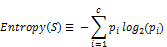
image003

image004

However, the information gain has a bias towards attributes with a high number of possible values (Mitchell, 1997). A way to overcome this bias is to select new selection attributes based on alternative criteria, such as the gain ratio (Quinlan, 1986), defined as:

image005

image006

In the GainRatio, the SplitInformation term attenuates the importance given to attributes with many, uniformly distributed, possible values.

Iterative Dichotomizer 3 (ID3)

The algorithm presented below is a slightly different version of the original ID3 algorithm as presented by Quinlan. The modifications are to support multiple output labels. In each recursion of the algorithm, the attribute which bests classifiers the set of instances (or examples, or input-output pairs, or data) is selected according to some selection criteria, such as the InfoGain or the GainRatio.

  • ID3(instances, target_attribute, attributes)
    • Create a new root node to the tree.
    • If all instances have the target_attribute belonging to the same class c,
      • Return the tree with single root node with label c.
    • If attributes is empty, then
      • Return the tree with single root node with the most common label of the target_attribute in instances.
    • Else
      • A ← the attribute in attributes which best classifies instances
      • root decision attribute ← A
      • Foreach possible value vi of A,
        • Add a new ramification below root, corresponding to the test A = vi
        • Let instancesvi be the subset of instances with the value vi for A
        • If instancesvi is empty then
          • Below this ramification, add a new leaf node with the most common value of target_attribute in instances.
        • Else below this ramification, add the subtree given by the recursion:
                  ID3(instancesvi, target_attribute, attributes – { A })
    • End
  • Return root

Difficulties and disadvantages of decision tree learning

Despite relying on the Occam’s Razor to guide the learning, neither ID3 or C4.5 algorithms are not guaranteed to produce the smaller or more general tree possible. This happens because their learning is based solely on heuristics and not in truly optimality criteria. The following example, from (Esmeir & Markovitch, 2007) illustrates the learning of the concept xor (exclusive or) by the ID3 algorithm. In this example, A3 and A4 are irrelevant attributes, having absolutely no influence on the target answer. However, yet being irrelevant, ID3 will select one of them to belong to the tree. In fact, ID3 will select the irrelevant attribute A4 to be the root of the learned tree.


A1 A2 A3 A4 label
1 0 0 1 +
0 1 0 0 +
0 0 0 0 -
1 1 0 0 -
0 1 1 1 +
0 0 1 1 -
1 0 1 1 +


image


One complication of decision tree learning is that the problem to find the smaller consistent tree (in the sense of classifying correctly all training samples) is known to be NP-complete (Hyafil & Rivest, 1976). Moreover, the separating decision surface generated by such trees are always formed by parallel cuts alongside the attribute space axis, which could be a severely suboptimal solution (Bishop, 2007, p. 666). The example given by Bishop illustrates well this problem: for example, to separate classes whose optimum decision margin are on 45 degrees from one of the axis, it will be needed a high number of parallel cuts in comparison with a single cut on the diagonal such as could be given by any linear decision machine. Another disadvantage of traditional decision tree learning algorithms is that most methods require only a constant learning time, and, as such, do not allow for trading extra training time for a better solutions. The work of (Esmeir & Markovitch, 2007) is dedicated to overcome such problem.

The following picture shows an example on how learning by decision trees is limited to cuts parallel to the axis, as described by Bishop. The Ying-Yang classification problem is a classical example of a non-linearly separable decision problem. Decision trees, albeit not being linear classifiers, have difficulty classifying this set with simple thresholds.

data-closerdecision-closertree

Top-Left: Ying-Yang non-linear classification problem. Top-Right: Decision surface extracted by a decision tree. Bottom: Decision threshold rules extracted from the tree.

However, despite all of those shortcomings, decision trees plays major roles as base of many successful algorithms. One interesting application and of notorious success is given in the field of object detection in images. The first real-time face detecting algorithm (Viola & Jones, 2001) is based on a degenerated decision tree (also known as a cascade). The body recognition and segmentation algorithm used by the Xbox 360 gaming platform used to process depth images generated by its companion sensor Kinect is equally based on the use of decision trees (Shotton, et al., 2011). As well is the case of the FAST algorithm for interest point detection in images (Rosten & Drummond, 2006).

I should also make the note that both the Viola-Jones and the FAST algorithms are available in the Accord.NET Framework for immediate use (the Viola-Jones (HaarObjectDetector) has also been recently updated to support multiple threads, so feel free to take a look and experiment with it!).

In sum, its possible to say that great part of the applicability of decision trees came from the simple fact that they are extremely fast to evaluate. One of the reasons for this feature is being easily translated to sets of conditional instructions in a conventional computer program. The decision trees now available in the Accord.NET Framework make full use of this fact and enables the user to actually compile the decision trees to native code on-the-fly, augmenting even more its performance during classification.

Source code

The code presented in this section is actually part of the Accord.NET Framework. The Accord.NET Framework is a framework extension to the already very popular AForge.NET Framework, adding and providing new algorithms and techniques for machine learning, computer vision and even more.

The Accord.MachineLearning.DecisionTree namespace is comprised of the following classes:

  • DecisionTree, the main class representing a decision tree, with methods such as Compute to compute the tree classification given an input vector;
  • DecisionNode, the node class for the decision tree, which may or may not have children nodes contained under a collection of children represented by a DecisionBranchNodeCollection;
  • DecisionVariable, a class to specify the nature of each variable processable by the tree, such as if the variable is continuous, discrete, which are their expected or valid ranges;
  • DecisionBranchNodeCollection, a class to contain children nodes together with information about which attribute of the data should be compared with the child nodes during reasoning.


Whose relationships can be seen in the following class diagram:

class diagram

The learning algorithms available are either the ID3 algorithm discussed above, or its improved version C4.5 (which can handle continuous variables, but at this time does not yet support pruning), both proposed and published by Ross Quinlan.

learning

Despite the bit complicated look, usage is rather simple as it will be shown in the next section.

Using the code

Consider, for example, the famous Play Tennis example by Tom Mitchell (1998):


  DataTable data = new DataTable("Mitchell's Tennis Example");
 
  data.Columns.Add("Day", "Outlook", "Temperature", "Humidity", "Wind", "PlayTennis");
 
  data.Rows.Add(   "D1",   "Sunny",      "Hot",       "High",   "Weak",    "No" );
  data.Rows.Add(   "D2",   "Sunny",      "Hot",       "High""Strong",   "No" );
  data.Rows.Add(   "D3""Overcast",    "Hot",       "High",   "Weak",    "Yes" );
  data.Rows.Add(   "D4",   "Rain",       "Mild",      "High",   "Weak",    "Yes" );
  data.Rows.Add(   "D5",   "Rain",       "Cool",     "Normal""Weak",    "Yes" );
  data.Rows.Add(   "D6",   "Rain",       "Cool",     "Normal", "Strong",   "No" );
  data.Rows.Add(   "D7""Overcast",    "Cool",     "Normal", "Strong",   "Yes" );
  data.Rows.Add(   "D8",   "Sunny",      "Mild",      "High",   "Weak",    "No" ); 
  data.Rows.Add(   "D9",   "Sunny",      "Cool",     "Normal""Weak",    "Yes" );
  data.Rows.Add(   "D10", "Rain",        "Mild",     "Normal""Weak",    "Yes" );
  data.Rows.Add(   "D11""Sunny",      "Mild",     "Normal", "Strong",   "Yes" );
  data.Rows.Add(   "D12", "Overcast",    "Mild",      "High""Strong",   "Yes" );
  data.Rows.Add(   "D13", "Overcast",    "Hot",      "Normal""Weak",    "Yes" );
  data.Rows.Add(   "D14""Rain",       "Mild",      "High""Strong",   "No" );


In the aforementioned example, one would like to infer if a person would play tennis or not based solely on four input variables. Those variables are all categorical, meaning that there is no order between the possible values for the variable (i.e. there is no order relationship between Sunny and Rain, one is not bigger nor smaller than the other, but are just distinct). Moreover, the rows, or instances presented above represent days on which the behavior of the person has been registered and annotated, pretty much building our set of observation instances for learning.


In order to try to learn a decision tree, we will first convert this problem to a more simpler representation. Since all variables are categories, it does not matter if they are represented as strings, or numbers, since both are just symbols for the event they represent. Since numbers are more easily representable than text string, we will convert the problem to use a discrete alphabet through the use of a codebook.


A codebook effectively transforms any distinct possible value for a variable into an integer symbol. For example, “Sunny” could as well be represented by the integer label 0, “Overcast” by “1”, Rain by “2”, and the same goes by for the other variables. So:


  // Create a new codification codebook to 
// convert strings into integer symbols
Codification codebook = new Codification(data);


Now we should specify our decision tree. We will be trying to build a tree to predict the last column, entitled “PlayTennis”. For this, we will be using the “Outlook”, “Temperature”, “Humidity” and “Wind” as predictors (variables which will we will use for our decision). Since those are categorical, we must specify, at the moment of creation of our tree, the characteristics of each of those variables. So:


  DecisionVariable[] attributes =
  {
    new DecisionVariable("Outlook",   3), // 3 possible values (Sunny, overcast, rain)
    new DecisionVariable("Temperature", 3), // 3 possible values (Hot, mild, cool)  
    new DecisionVariable("Humidity", 2), // 2 possible values (High, normal)   
    new DecisionVariable("Wind", 2) // 2 possible values (Weak, strong)
  };


  int classCount = 2; // 2 possible output values for playing tennis: yes or no


Let's now proceed and create our DecisionTree:


  DecisionTree tree = new DecisionTree(attributes, classCount); 


Now we have created our decision tree. Unfortunately, it is not really very useful, since we haven't taught it the problem we are trying to predict. So now we must instantiate a learning algorithm to make it useful. For this task, in which we have only categorical variables, the simplest choice is to use the ID3 algorithm by Quinlan. Let’s do it:


// Create a new instance of the ID3 algorithm
ID3Learning id3learning = new ID3Learning(tree);

// Translate our training data into integer symbols using our codebook:
DataTable symbols = codebook.Apply(data);
int[][] inputs = symbols.ToIntArray("Outlook", "Temperature", "Humidity", "Wind");
int[] outputs = symbols.ToIntArray("PlayTennis").GetColumn(0);

// Learn the training instances!
id3learning.Run(inputs, outputs);


At this point, the tree has been created. A suitable representation of the learned tree could be given by the following diagram:


image


However, more than just a diagram, we can also go and generate a .NET Expression Tree describing our decision tree. Expression trees represent code in the form of a tree of expressions, which can then be read, modified or compiled. By compiling the DecisionTree's expression, we are able to generate code on-the-fly and let the JIT compile it down to native code at runtime, greatly improving the performance of our decision tree:


  // Convert to an expression tree
var expression = tree.ToExpression();
 
  // Compiles the expression to IL
var func = expression.Compile();


And here is the resulting C# code obtained by compiling the expression into a lambda function, dumping the function into an dynamic assembly, opening and inspecting this assembly using ILSpy:


  public static int Compute(double[] input)
  {
    if (input[0] == 0.0)
    {
      if (input[2] == 0.0)
      {
        return 0;
      }
      if (input[2] == 1.0)
      {
        return 1;
      }
      throw new ArgumentException(
        "Input contains a value outside of expected ranges.", "input"); 
    }
    else 
    {
      if (input[0] == 1.0)
      {    return 1;
      }
      if (input[0] != 2.0)
      {
        throw new ArgumentException(
          "Input contains a value outside of expected ranges.", "input");
      }
      if (input[3] == 0.0)
      { 
        return 1;  
      }
      if (input[3] == 1.0)
      {
        return 0;
      }
      throw new ArgumentException(
        "Input contains a value outside of expected ranges.", "input");
    }
  }


I suspect I should have included more input validation on the generated code. However, the release is now closed and will be made available for download soon. If there is need, more robust code generation may added as a feature in later versions.


Conclusion


Decision trees are useful tools when the problem to be solved needs to be quickly interpreted and understood by humans. Another suitable use is when the decision needs to be fast. However, decision trees, at least those trained by simple training algorithms such as ID3 and C4.5 can perform quite poorly depending on the problem. As it happens with all machine learning techniques, it is futile to believe there is a one true classifier which would act perfectly on all possible imaginable scenarios. As always, it is important to know our tools and know in which situation each technique would work better.


References


  • Bishop, C. M., 2007. Pattern Recognition and Machine Learning (Information Science and Statistics). 1st ed. 2006. Corr. 2nd printing ed. s.l.:Springer


  • Fayyad, U. M. & Irani, K. B., 1992. On the Handling of Continuous-Valued Attributes in Decision Tree Generation. Machine Learning, January, 8(1), pp. 87-102.


  • Quinlan, J. R., 1986. Induction of decision trees. Machine Learning, 1(1), pp. 81-106.


  • Quinlan, J. R., 1993. C4.5: Programs for Machine Learning (Morgan Kaufmann Series in Machine Learning). 1 ed. s.l.:Morgan Kaufmann.


  • Shotton, J. et al., 2011. Real-Time Human Pose Recognition in Parts from Single Depth Images. s.l., s.n.


  • Viola, P. & Jones, M., 2001. Robust Real-time Object Detection. s.l., s.n.


  • Mitchell, T. M., 1997. Decision Tree Learning. In:: Machine Learning (McGraw-Hill Series in Computer Science). s.l.:McGraw Hill.


  • Mitchell, T. M., 1997. Machine Learning (McGraw-Hill Series in Computer Science). Boston(MA): WCB/McGraw-Hill.


  • Esmeir, S. & Markovitch, S., 2007. Anytime Learning of Decision Trees. J. Mach. Learn. Res., May, Volume 8, pp. 891-933.


  • Hyafil, L. & Rivest, R. L., 1976. Constructing Optimal Binary Decision Trees is NP-complete. Information Processing Letters, 5(1), pp. 15-17.

Friday, 1 July 2011

Accord.NET Framework: Gesture Controller Components

A new version (2.2.0) of the Accord.NET Framework has just been released. This new version introduces many new features, fixes and improvements. The most interesting additions are certainly the HeadController and FaceController .NET components.


Accord.NET Framework sample application for Gesture Controller Components

The Accord.NET Controller components can be used to generate events based on webcam motion. By using a combination of HaarCascadeClassifiers, Camshift and Template-based Tracking, those components are able to detect when a face enters scene, leaves the scene, and moves across a scene.

The video above shows only the sample application which comes together with the framework. However, the interesting part is that this is just a sample of what can be accomplished using the real controller components. The controller components are .NET components, similar to Button, Label or Timer, and can be dragged and dropped from Visual Studio’s ToolBox directly into any application.

Accord.NET Controller Components in Visual Studio

Once inside an application, it will be possible to set event actions just as in any other .NET component:

Setting events for head movements using Accord.NET Controller Components

The controls have built-in support for calibration. All values except tilting angle are passed to the hosting application in the [-1;+1] range, in which -1 indicates either a total left/down/backwards position and +1 indicates a total right/up/forward position. The tilting angle is given in radians. Please note that the face controller is still a bit experimental and still requires some tuning.


This new version also introduces HSL Color Range object trackers, more default Haar Cascades, an experimental version of linear-chain Conditional Random Fields, and the ability to generate hardcoded C# definitions of any Haar cascade available in the OpenCV XML format. There is also initial support for finger detection using new implementations for Border-Following contour extraction, K-Curvatures and Convex Hull Defects extraction. On the statistics side, there has been the inclusion of the Von-Mises distribution, Moving and Running Normal distributions and improvements in the Multivariate Gaussian implementation. The full release notes are available in the release's download page.

Also, a special thanks to Professor Dr. Modesto Castrillón Santana to let me embed some of his Haar definitions into the framework under the LGPL license. Please be sure to include a reference to his work if you plan to use this in an academic publication.


As always, I hope those additions and improvements will be useful to everyone :-)

Monday, 29 November 2010

Machine Learning Books and Lectures

Jordan, one of the readers of the blog, wrote to point out some cool references for machine learning, mathematics and artificial intelligence.

Thanks again for all your contributions. I'm a .NET programmer coming from a background of studying politics and Latin American studies so when the moment came that I realized I was interested in A.I., I didn't have many resources to turn to.

I have a collection of books and links that I found very very helpful when I was trying to learn about these concepts. I was thinking they could be useful to some of your readers who were in my shoes two years ago. So without further adieu:


Handbook of Normal Frames and Coordinates

"Handbook of Normal Frames and Coordinates," Iliev, Bozhidar Z. (2006)

“This can be a heavy text, but if you understand the concept, this can take you to the next level - I would categorize this as Topology but has applications in quantum physics, theoretical mathematics, theoretical physics etc...- in context of your blogs - granted this is a dedicated read - I think readers will be able to appreciate and truly understand what a Hilbert Space is after reading this book.”

Linear Algebra

"Linear Algebra," Jim Heffron (2008)

“I liked this one because it was free and is still highly rated - I have also heard great reviews about David Poole's book on linear algebra, but I couldn't get myself to shell out the money when this was free.”

Complex To Real

http://www.complextoreal.com/tutorial.htm

“There are a ton of great articles here - I have personally read the ones on fourier transforms and wavelet transforms - great stuff”

Stanford Lectures - Fourier Analysis series

(free through Youtube or iTunesU)

“Email the Professor for the companion book. At this point it may have been published - but well worth shelling out the dough in any case.”

Bio-Inspired Artificial Intelligence

"Bio-Inspired Artificial Intelligence," Floreano and Mattiussi (2008)

“Excellent reference - fairly in depth for the number of topics it covers, lots of illustrations (illustrations are always a good thing :) and I've also found it to be a useful source for inspiration. I bought this book while I was looking into fuzzy swarm intelligence - it doesn't have all the answers, but I am simply in love with this book.”

Video lectures on Machine Learning

http://videolectures.net/pascal/

“A collection of video lectures featuring very brilliant people - let's face it... if you're doing or are interested in mathematics this complex... you probably don't know too many people who you can talk to / learn from on the subject unless you're in a University studying this kind of thing - these are some great lectures on machine learning - I just recently found this site but wish I had found it sooner - it's great if you're just exploring machine learning or are very well versed in it - however, I fall somewhere in the middle of that distribution so take it for what it's worth!”

Fearless Symmetry

"Fearless Symmetry," Ash and Gross (2006)

Another accessible book to those without heavy training in math - great intro to Galois Theory, the Riemann Hypothesis and several other concepts.

Zero: The Biography of a Dangerous Idea

    "Zero: The Biography of a Dangerous Idea," Charles Seife (2000)

This one is more historical and conceptual than technical but it's a captivating read and will help get you through those hard times when you want to put down that book on K-Dimensional Manifolds, but still need to satisfy your mathematical mind (some say it's never at rest once you catch that "learning bug").

Khan Academy

http://www.khanacademy.org/

Finally,  when you get lost, go here! The Khan Academy is a not-for-profit 501(c)(3) with the mission of providing a world-class education to anyone, anywhere.


Thanks Jordan! I hope readers can enjoy those resources as much as I did. Cheers!

Monday, 18 October 2010

Gaussian Mixture Models and Expectation-Maximization

Like K-Means, Gaussian Mixture Models (GMM) can be regarded as a type of unsupervised learning or clustering methods. They are among the most statistically mature methods for clustering. But unlike K-Means, GMMs are able to build soft clustering boundaries, i.e., points in space can belong to any class with a given probability.


The code presented here is also part of the Accord.NET Framework. The Accord.NET Framework is a framework for developing machine learning, computer vision, computer audition, statistics and math applications. It is based on the already excellent AForge.NET Framework. Please see the starting guide for mode details. The latest version of the framework includes the latest version of this code plus many other statistics and machine learning tools.

Contents


gaussians


  1. Introduction

  2. Source code

    1. Normal Distributions

    2. Mixture Distributions

    3. Expectation-Maximization

    4. Gaussian Mixture Models


  3. Using the code

  4. Sample application

  5. Conclusion

  6. References

  7. See also


Introduction


In statistics, a mixture model is a probabilistic model which assumes the underlying data to belong to a mixture distribution. In a mixture distribution, its density function is just a convex combination (a linear combination in which all coefficients or weights sum to one) of other probability density functions:


The individual pi(x) density functions that are combined to make the mixture density p(x) are called the mixture components, and the weights w1, w2, …, wn associated with each component are called the mixture weights or mixture coefficients.


The most common mixture distribution is the Gaussian (Normal) density function, in which each of the mixture components are Gaussian distributions, each with their own mean and variance parameters.


To give a more solid and concrete understanding of the Gaussian mixture models, we will be jumping directly on how to represent those abstractions in source code through the use of class diagrams. Hopefully class diagrams may give a better and direct overview on the subject than a lengthy theoretical discussion.


Source code


First we will discuss about the characteristics of any probability distribution. The IDistribution interface (depicted below) says any probability distribution may have a probability function and a distribution function. It also says that probability distributions can also be fitted to sets of observations through a parameter estimation method.


IDistribution


Since distribution functions can be either univariate or multivariate, the methods above accept any number of scalar values as input through the use of the params keyword. The Fit method for parameter estimation also accepts a general System.Array because we could be given either an array of univariate observations in the form of a double[] or an array of multivariate observations in the form of a jagged double[][] array. Since each observation may have a different weight in the estimation process, the weights parameter can be used to inform those weights to the fitting method.


Probability distributions may also have some associated measures, mainly the Expectation and the Variance of the modeled random variable. Depending if the distribution is univariate or multivariate, the expected values and variances can be either a single scalar or a vector of scalars. For multivariate distributions the variance can be also represented by a symmetric, positive-definite matrix known as the variance-covariance matrix.


IDistributions


Moreover, probability distributions can also be continuous or discrete. In continuous distributions the probability function is known as the Probability Density Function (pdf), and in discrete distributions the probability function is known as the Probability Mass Function (pmf). However, since our distribution of interest, the Gaussian, is a continuous distribution, be focusing only on continuous multivariate distributions:


All


The Normal (Gaussian) distribution and the mixture distributions fall under the multivariate continuous distributions category and are implemented as such.


Normal distributions


The Normal (or Gaussian) multivariate distribution is a multivariate distribution whose parameters are the mean vector μ and a variance-covariance matrix Σ. Its probability density function is given by:


The more detailed class diagram for the normal distribution shows the multivariate characteristics of most of its methods, in particular of the Fit method for estimating Gaussian parameters from a multivariate set of data. Each sample, given in the form of a double[], may also have different associated weights. In this case, the weight associated with each of the samples can be passed through the weights parameter.


NormalDistribution

To estimate the parameters of a Gaussian distribution all we have to do is compute the mean and the variance-covariance matrix out of the given data. This is a very straightforward procedure and can be done by using the standard methods of the Tools class in the Accord.Statistics namespace. The Fit method returns the fitted distribution as a return value and leaves the current distribution untouched.


Mixture distributions


Mixture distributions are just convex combinations of other probability distributions. Thus said, mixture distributions have an array of component distributions and a coefficient array which contains the weights of the each of the component probability distributions.


Mixture


In the generic implementation above, T is the type of the distributions used in the mixture. The most common mixture distribution, the Gaussian Mixture Distribution, could then be created by instantiating a Mixture<NormalDistribution> object passing the initial Normal distributions as constructor parameters.


Alternatively, the parameters of the mixture distributions could be estimated from a set of observations by calling the Fit method. To estimate the parameters of a mixture distribution we will be using a common technique known as the Expectation-Maximization algorithm.


Expectation Maximization


Expectation-Maximization (EM) is a well established maximum likelihood algorithm for fitting a mixture model to a set of training data. It should be noted that EM requires an a priori selection of model order, namely, the number of M components to be incorporated into the model.


The general E-M algorithm is comprised of the following simple steps:


  1. Initialization

    Initialize the distribution parameters, such as the means, covariances and mixing coefficients and evaluate the initial value of the log-likelihood (the goodness of fit of the current distribution against the observation dataset)’;

  2. Expectation

    Evaluate the responsibilities (i.e. weight factors of each sample) using the current parameter values;

  3. Maximization

    Re-estimate the parameters using the responsibilities found in the previous step;

  4. Repeat

    Re-evaluate the log-likelihood and check if it has changed; if it has changed less than a given threshold, the algorithm has converged.


Below is the actual realization of the algorithm as implemented in the Fit method of the Mixture<T> class.


/// <summary>
/// Fits the underlying distribution to a given set of observations.
/// </summary>
///
/// <param name="observations">The array of observations to fit the model against. The array
/// elements can be either of type double (for univariate data) or
/// type double[] (for multivariate data).</param>
/// <param name="weights">The weight vector containing the weight for each of the samples.</param>
/// <param name="options">Optional arguments which may be used during fitting, such
/// as regularization constants and additional parameters.</param>
///
/// <remarks>
/// Although both double[] and double[][] arrays are supported,
/// providing a double[] for a multivariate distribution or a
/// double[][] for a univariate distribution may have a negative
/// impact in performance.
/// </remarks>
///
public override void Fit(double[] observations, double[] weights, IFittingOptions options)
{
// Estimation parameters
double threshold = 1e-3;
IFittingOptions innerOptions = null;

if (options != null)
{
// Process optional arguments
MixtureOptions o = (MixtureOptions)options;
threshold = o.Threshold;
innerOptions = o.InnerOptions;
}


// 1. Initialize means, covariances and mixing coefficients
// and evaluate the initial value of the log-likelihood

int N = observations.Length;
int K = components.Length;

double weightSum = weights.Sum();

// Initialize responsabilities
double[] norms = new double[N];
double[][] gamma = new double[K][];
for (int k = 0; k < gamma.Length; k++)
gamma[k] = new double[N];


// Clone the current distribution values
double[] pi = (double[])coefficients.Clone();
T[] pdf = new T[components.Length];
for (int i = 0; i < components.Length; i++)
pdf[i] = (T)components[i].Clone();

// Prepare the iteration
double likelihood = logLikelihood(pi, pdf, observations, weights);
bool converged = false;

// Start
while (!converged)
{
// 2. Expectation: Evaluate the component distributions
// responsibilities using the current parameter values.
Array.Clear(norms, 0, norms.Length);

for (int k = 0; k < gamma.Length; k++)
for (int i = 0; i < observations.Length; i++)
norms[i] += gamma[k][i] = pi[k] * pdf[k].ProbabilityFunction(observations[i]);

for (int k = 0; k < gamma.Length; k++)
for (int i = 0; i < weights.Length; i++)
if (norms[i] != 0) gamma[k][i] *= weights[i] / norms[i];

// 3. Maximization: Re-estimate the distribution parameters
// using the previously computed responsibilities
for (int k = 0; k < gamma.Length; k++)
{
double sum = gamma[k].Sum();

for (int i = 0; i < gamma[k].Length; i++)
gamma[k][i] /= sum;

pi[k] = sum / weightSum;
pdf[k].Fit(observations, gamma[k], innerOptions);
}

// 4. Evaluate the log-likelihood and check for convergence
double newLikelihood = logLikelihood(pi, pdf, observations, weights);

if (Double.IsNaN(newLikelihood) || Double.IsInfinity(newLikelihood))
throw new ConvergenceException("Fitting did not converge.");

if (Math.Abs(likelihood - newLikelihood) < threshold * Math.Abs(likelihood))
converged = true;

likelihood = newLikelihood;
}

// Become the newly fitted distribution.
this.initialize(pi, pdf);
}


Gaussian Mixture Models


Gaussian mixture models are among the most commonly used examples of mixture distributions. The GaussianMixtureModel class encompasses a Mixture<NormalDistribution> object and provides methods to learn from data and to perform actual classification through a simplified interface.


Class diagram for Gaussian Mixture Model


Moreover, a common problem which rises in mixture model fitting through E-M is the proper initialization of the mixture parameters. One popular approach is to initialize the mixture parameters using the centroids detected by the K-Means algorithm. The code below shows how the mixture parameters are computed by first creating a KMeans object and then passing the clusters to the mixture model for further processing.


    /// <summary>
/// Divides the input data into K clusters modeling each
/// cluster as a multivariate Gaussian distribution.
/// </summary>
public double Compute(double[][] data, double threshold)
{
int components = this.gaussians.Count;

// Create a new K-Means algorithm
KMeans kmeans = new KMeans(components);

// Compute the K-Means
kmeans.Compute(data, threshold);

// Initialize the Mixture Model with data from K-Means
NormalDistribution[] distributions = new NormalDistribution[components];
double[] proportions = kmeans.Clusters.Proportions;
for (int i = 0; i < components; i++)
{
double[] mean = kmeans.Clusters.Centroids[i];
double[,] covariance = kmeans.Clusters.Covariances[i];
distributions[i] = new NormalDistribution(mean, covariance);
}

// Fit a multivariate Gaussian distribution
model = Mixture<NormalDistribution>.Estimate(data, threshold, proportions, distributions);

// Return the log-likelihood as a measure of goodness-of-fit
return model.LogLikelihood(data);
}


Using the code


Code usage is rather simple. First, instantiate a new GaussianMixtureModel object passing the desired number of components in the Gaussian mixture. Then, call the Compute(double[][], double) method passing the learning samples and a desired convergence threshold.


// Create a new Gaussian Mixture Model with 2 components
GaussianMixtureModel gmm = new GaussianMixtureModel(2);

// Compute the model (estimate)
gmm.Compute(samples, 0.0001);

// Classify a single sample
int c = gmm.Classify(sample);


After training has been completed, a new sample can be classified by calling the Classify(double[]) method.


Sample application


The accompanying sample application demonstrates how Gaussian Mixture Models can be used to cluster normally-distributed samples of data. By clicking the “Create random data” button, a given number of Normal distributions will be created in the two-dimensional space using random mean and covariance matrices.


After the data has been created, you can use the “Fit a Gaussian Mixture Model” button to fit a mixture of Gaussians to the data. Each of the Gaussians will receive a random color and the samples which have the greatest probability of belonging to any of the Gaussians will be colored accordingly.


Sample7 Sample8


Left: a random dataset containing three Gaussian clusters. Right: the clusters as identified by the Gaussian Mixture Model.


Sample9 Sample10


Left: a random dataset containing 10 Gaussian clusters. Right: the clusters as identified by the Gaussian Mixture Model.


Conclusion


In this article we found how Gaussian Mixture Models can be successfully used to create soft clustering boundaries around data. Those soft boundaries are possible because in a mixture model each sample is said to belong to a cluster only within certain probability.


A main drawback of GMMs is that the number of Gaussian mixture components, as in K-Means, is assumed known as prior, so it cannot be considered as totally unsupervised clustering method. To aid in this situation, one could use additional algorithms such as the Minimum Message Length(MML) criteria.


Another problem arises with the correct initialization of the mixture components. A poor choice of initial parameters will invariably lead to poor results, as the E-M algorithm converges only to a local optimization point. A commonly used solution is initialization by randomly sampling in the mixture data. Other common solution, covered by the implementation presented here, is to use K-Means to perform initialization. However, K-Means itself may also converge to a poor solution and impact negatively in the mixture model fitting.


References


  • Raja, Y., Shaogang, G. Gaussian Mixture Models. Department of Computer Science, Queen Mary and Westfield College, England.


  • Bishop, C. M. (2007), Pattern Recognition and Machine Learning (Information Science and Statistics), Springer.


  • Wikipedia contributors, "Normal distribution," Wikipedia, The Free Encyclopedia, http://en.wikipedia.org/w/index.php?title=Normal_distribution (accessed October 18, 2010).


  • Wikipedia contributors, "Probability density function," Wikipedia, The Free Encyclopedia, http://en.wikipedia.org/w/index.php?title=Probability_density_function (accessed October 18, 2010).


  • Wikipedia contributors, "Mixture density," Wikipedia, The Free Encyclopedia, http://en.wikipedia.org/w/index.php?title=Mixture_density (accessed October 18, 2010).


See also